The 10-Second Trick For Excel Jobs

By pushing ctrl+change+facility, this will certainly determine and also return value from numerous arrays, instead than just private cells included in or multiplied by each other. Calculating the sum, item, or ratio of private cells is very easy-- just make use of the =AMOUNT formula and enter the cells, values, or variety of cells you intend to execute that arithmetic on.

If you're wanting to discover overall sales income from a number of marketed units, for instance, the selection formula in Excel is excellent for you. Right here's exactly how you would certainly do it: To begin utilizing the range formula, kind "=AMOUNT," and also in parentheses, go into the very first of two (or three, or 4) ranges of cells you would love to multiply together.

This stands for reproduction. Following this asterisk, enter your 2nd range of cells. You'll be increasing this 2nd series of cells by the very first. Your progression in this formula should now resemble this: =AMOUNT(C 2: C 5 * D 2:D 5) Ready to push Go into? Not so fast ... Because this formula is so difficult, Excel gets a various keyboard command for arrays.

This will acknowledge your formula as a variety, covering your formula in brace characters as well as efficiently returning your item of both arrays integrated. In income computations, this can reduce your time and initiative considerably. See the last formula in the screenshot over. The MATTER formula in Excel is signified =MATTER(Start Cell: End Cell).

For instance, if there are 8 cells with gotten in values in between A 1 as well as A 10, =MATTER(A 1: A 10) will return a worth of 8. The MATTER formula in Excel is specifically valuable for large spread sheets, wherein you intend to see the number of cells consist of actual entrances. Don't be deceived: This formula will not do any type of mathematics on the worths of the cells themselves.

4 Easy Facts About Learn Excel Shown

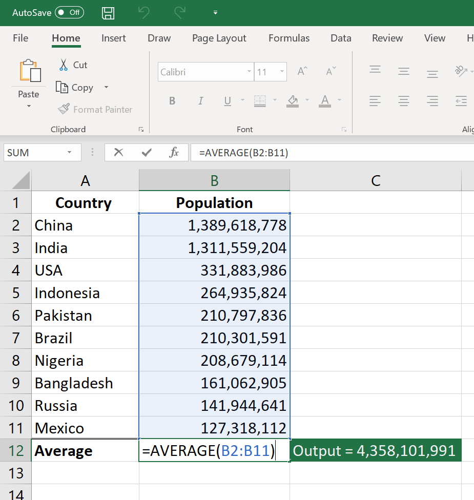
Making use of the formula in strong over, you can easily run a matter of active cells in your spreadsheet. The result will certainly look a little something such as this: To execute the typical formula in Excel, go into the values, cells, or variety of cells of which you're computing the average in the layout, =AVERAGE(number 1, number 2, etc.) or =STANDARD(Beginning Worth: End Value).

Finding the average of a variety of cells in Excel maintains you from having to discover individual amounts and also then carrying out a different division equation on your total amount. Using =AVERAGE as your initial message access, you can allow Excel do all the job for you. For reference, the standard of a team of numbers amounts to the amount of those numbers, separated by the variety of products in that team.

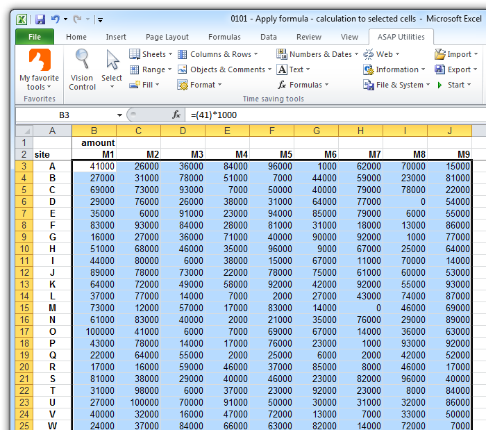
This will return the amount of the worths within a desired variety of cells that all fulfill one standard. For instance, =SUMIF(C 3: C 12,"> 70,000") would return the amount of values between cells C 3 as well as C 12 from just the cells that are more than 70,000. Let's say you desire to determine the revenue you produced from a list of leads who are related to specific location codes, or determine the sum of certain workers' salaries-- yet just if they fall over a specific quantity.

With the SUMIF feature, it doesn't need to be-- you can easily build up the sum of cells that meet particular requirements, like in the income example over. The formula: =SUMIF(range, requirements, [sum_range] Variety: The range that is being examined using your requirements. Requirements: The standards that identify which cells in Criteria_range 1 will certainly be totaled [Sum_range]: An optional series of cells you're mosting likely to build up along with the very first Range got in.

In the example below, we wished to determine the amount of the salaries that were better than $70,000. The SUMIF function accumulated the dollar amounts that surpassed that number in the cells C 3 with C 12, with the formula =SUMIF(C 3: C 12,"> 70,000"). The TRIM formula in Excel is denoted =TRIM(text).

The Ultimate Guide To Excel Jobs

As an example, if A 2 includes the name" Steve Peterson" with undesirable areas prior to the given name, =TRIM(A 2) would return "Steve Peterson" without any spaces in a new cell. Email and also submit sharing are terrific devices in today's work environment. That is, until among your colleagues sends you a worksheet with some truly cool spacing.

Rather than fastidiously eliminating as well as adding areas as needed, you can cleanse up any irregular spacing using the TRIM function, which is used to get rid of extra rooms from information (besides single rooms between words). The formula: =TRIM(message). Text: The message or cell where you wish to eliminate areas.

To do so, we entered =TRIM("A 2") into the Formula Bar, and duplicated this for each name below it in a brand-new column beside the column with unwanted rooms. Below are some other Excel formulas you might locate beneficial as your information management needs grow. Let's claim you have a line of text within a cell that you desire to break down into a few different sections.

Objective: Made use of to draw out the very first X numbers or characters in a cell. The formula: =LEFT(message, number_of_characters) Text: The string that you want to extract from. Number_of_characters: The number of personalities that you wish to extract beginning with the left-most character. In the example listed below, we got in =LEFT(A 2,4) into cell B 2, and also duplicated it right into B 3: B 6.

Function: Used to remove characters or numbers between based upon position. The formula: =MID(text, start_position, number_of_characters) Text: The string that you desire to remove from. Start_position: The placement in the string that you intend to begin extracting from. For instance, the first position in the string is 1.

The Basic Principles Of Excel Skills

In this instance, we got in =MID(A 2,5,2) right into cell B 2, as well as duplicated it right into B 3: B 6. That permitted us to remove the two numbers beginning in the 5th position of the code. Objective: Made use of to remove the last X numbers or personalities in a cell. The formula: =RIGHT(message, number_of_characters) Text: The string that you desire to remove from.

excel formulas equal formula excel irr excel formulas variable